Introduction

Buildings include commercial buildings, office buildings, and residential buildings. The unit area of energy consumption in residential buildings is small, but the total amount is large, thus, it cannot be ignored. For residential buildings, energy consumption is mainly due to the use of heating, electricity, ventilation (mechanical), and cooling from air conditioning systems (HVAC). The parameters that affect the energy consumption of residential buildings are the environment and the structure of the house. Environmental parameters include temperature, humidity, intensity of sunlight exposure, etc.

In order to learn the energy consumption and temperature behaviors of buildings, in this project we will focus on the building of “residential 2” in Rome and study the effect of the following parameters: window glazing (single, double, or triple), ventilation (on or off), shading (on or off), wall insulation thickness and roof insulation thickness. Due to the climate change throughout the year, we will also modify the settings or schedules of heating, cooling, and ventilation. In the end, we will propose the implementation of a series of models for the forecast of home energy consumption. In addition, some other analyses for Windows will be presented as well.

Target building description

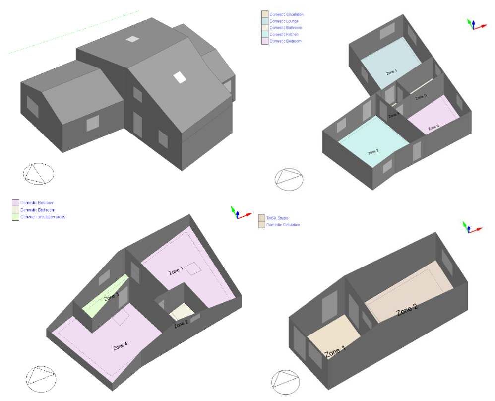
In our project, we focus on a residential building with the name “Residential2” and the weather of “Roma”. In the following figure, we can see that the house is composed of two components including one house with two floors and one office. In particular, on the one hand, we have on the ground floor one bedroom, one bathroom, one kitchen, and a lounge, and on the first floor, we have a relatively small area with one bedroom and one bathroom. On the other hand, the office has two rooms. Moreover, the location of the house is set to be Rome and so is the weather. Meanwhile, due to the different functions and requirements of the house and office, it is reasonable to consider them separately in terms of schedule. Note that, there is another area of the roof and it will not be taken into account.

In order to learn the behavior of overall (annual) energy consumption including electricity, heating, and cooling, based on different building elements, we use DesignBuilder to simulate the target building and generate idf file with the target weather data of Rome. In particular, we change the following parameters: window glazing (single, double, or triple), ventilation (on or off), and shading (on or off). In the meantime, we also modified the settings or schedules of heating, cooling, and ventilation. As a result, we generate multiple idf files for simulation through EnergyPlus. Then, we refer to besos to further change some parameters (e.g., wall insulation thickness) to see how the energy consumption varies with respect to the changing of parameters so that we are able to derive the combination of parameters for best performance (lowest energy consumption).

Visualization and Energy Signature

In our building, we simulate a situation that which there are sensors in each room to collect temperature data and meters to calculate the energy consumption, and send the data to the server via MQTT protocol, then the server writes the data in the database using the HTTP method. The data are collected over time, so we use InfluxDB as the database to store the time series data and use the Grafana dashboard for visualization.

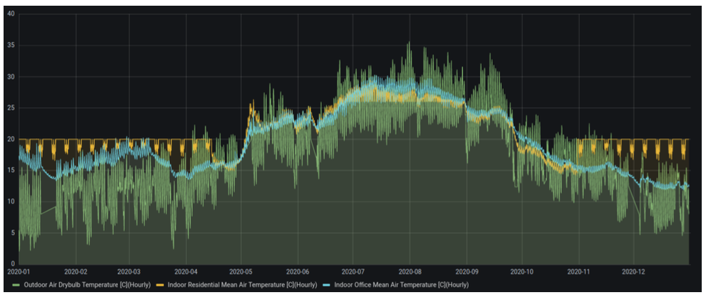
This figure shows the outdoor and indoor temperature over a year, where we show the indoor temperature of residential area and office areas separately. We can see that there is an obvious temperature difference between those two areas, especially in winter. It reflects the different heating and cooling schedules in different areas.

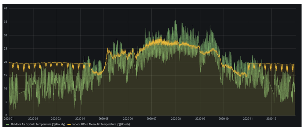
This figure shows the indoor weighted mean temperature, which allows us to see the difference from Figure 3-1, and we use the volume of each zone as the weight. It’s obvious that internal temperature and heating in winter have periodicity while the other 3 seasons don’t have this feature, which has an influence on later analysis. From this figure and the previous one, we are also able to see the periodicity of one week for heating in winter.

This figure shows the total energy consumption and the heating and cooling energy.

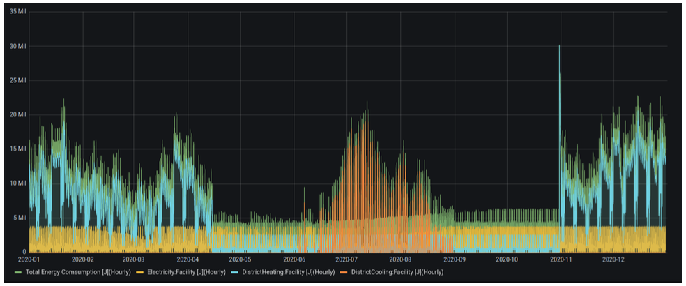
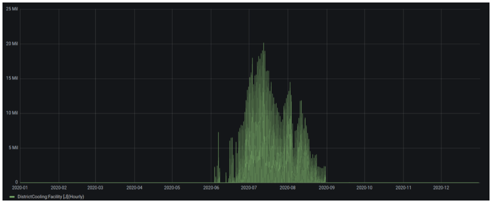
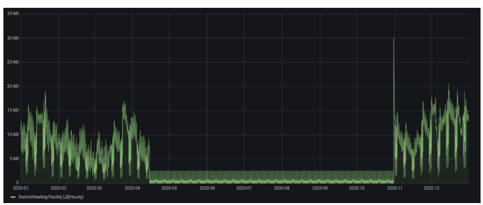
These figures show the heating and cooling energy used in 2020, and it’s easy to draw the conclusion that the cooling system functions only in summer, while the heating system only works in winter. Thus, according to this figure, we manually divided the whole year into 4 seasons, which are summer with a cooling system, winter with a heating system, and spring/fall with no heating and cooling consumption.

Prediction

LSTM

LSTM is short for Long Short-Term Memory, which is the development of the RNN. It is designed to capture the arbitrary time lag of the time series. Compared with the Prophet, which is researched below, LSTM is a black box and the shortage of data shall result in the relatively low performance.

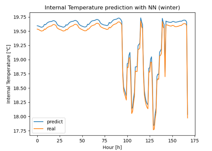
In the figure, the prediction based on the best parameters of LSTM is made, and due to the similarity of the figures and the brevity of the report, the rest method will not post all the figures about the prediction but only the internal temperature prediction in winter. The performance of the methods can be checked with the MSE table.

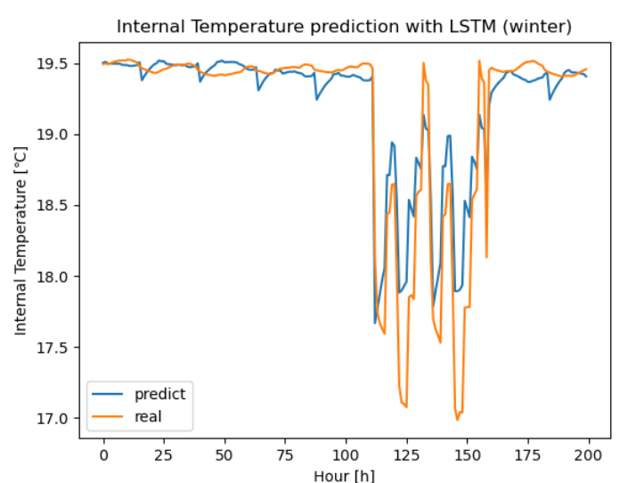
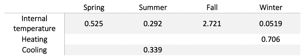
From the performance in this table, LSTM has a great performance in winter of predicting the internal temperature, but the performance in fall is quite low, it is may because of the unstable outdoor temperature of the fall. Nevertheless, the performance of LSTM is acceptable.

Regression neural network

The neural network is a computing system inspired by the biological neural network of animal brains. In 1958, it was first introduced by psychologist Frank Rosenblatt. Then the most important method “back propagation” was derived by Kelley in 1960. After that, there are many neural networks with different structures flourished, to solve different specific problems, including the LSTM mentioned above.

In this research, the normal neural network is the simplest method, working as linear regression in machine learning. The neural network will use outdoor air-dry bulb temperature and other data as regressands to find the linear relations. To make the prediction more precise, the internal temperature of last time unit is used because the temperature change is an integral process. The accuracy of the regression neural network is listed in the table and the prediction example is shown in the figure.

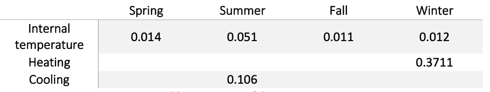
The performance of the basic neural network is relatively the steadiest of all the methods. This character may defer to the strong correlations between the regressors and the regressands. And for the prediction of a less time-reliable value such as the heating and cooling, it doesn’t behave as well as the temperature.

Hidden Markov model

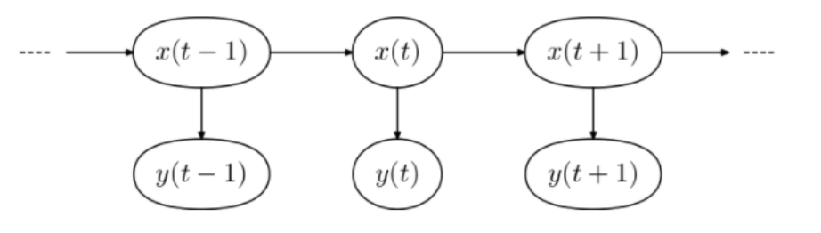
The hidden Markov model is a state space model that uses statistical property to describe the evolution based on existing and observable samples to derive the latent factors (hidden states) that are not directly observable. The general idea can be described in the following figure, samples of y are those observables while x are hidden states. Based on the knowledge of the sequence of y, we derive the sequence of hidden states, and as a result, we are able to get the most probable state of the next time instance with maximum probability and thus, get the prediction of y. In our case, due to the periodicity of one week, we use 7 days (24*7=168 samples) to predict the value of the next hour and repeat the procedure for 200 samples for internal temperature during winter as well as summer, heating, and cooling energy consumption. On the other hand, we will refer to a Python package named “hmmlearn” to implement a hidden Markov model.

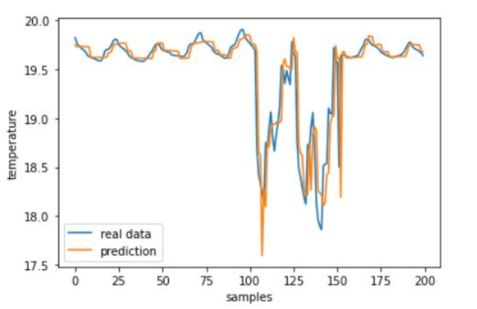
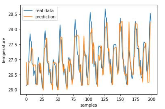
In the following figure, we can see the prediction of internal temperature in winter versus real data. Generally speaking, despite the fact that the two lines do not coincide with each other perfectly, the predictions are still able to follow the trend of real data and identify the periodicity during the day as well as the week. However, it cannot be ignored that the peak hour has a large variance with respect to real data.

On the other hand, we also have learned the internal temperature evolution in summer and the result is in the following figure. In general, the prediction can still follow the trend of real data but the peaks are even harder to be predicted with respect to those in winter and as a consequence, the performance of prediction is not good.

Meanwhile, the predictions of heating and cooling energy consumption are also performed and the results can be seen in the following figure.

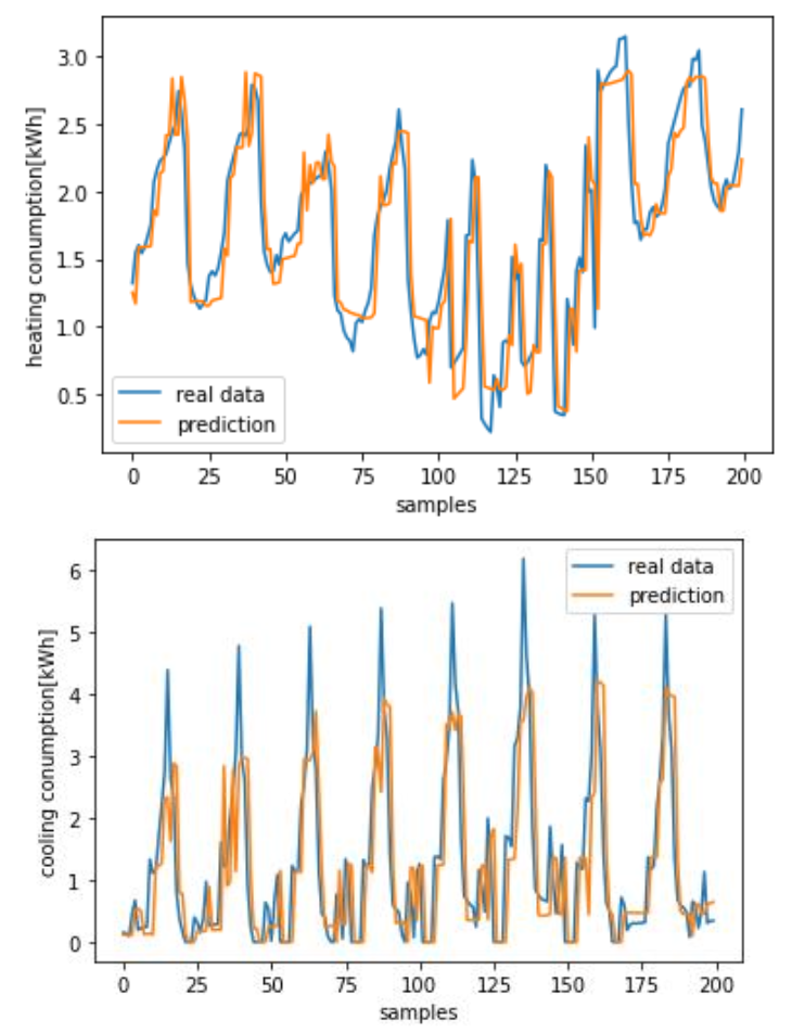
Similar to the previous condition of internal temperature in winter and summer, the performance of heating consumption is better than that of cooling consumption. The presence of strong peaks due to dramatic changes in values results in difficulties in prediction.

Statistically speaking, the R2 score for prediction in summer is poor while it is somewhat decent for prediction in winter, but the overall results are merely acceptable and the prediction is able to follow the trend of real data. In particular, the hidden Markov model is not a perfect tool in our specific case since the prediction strongly correlates to the values of previous samples.

Prophet

Prophet is a time series analysis tool publicized by Facebook in 2017 and we chose it because of its flexibility. The seasonal trend with different periods can be easily introduced, and the missing value will be automatically fixed before the fitting, which is impossible for the traditional model such as ARIMA. Similar to ARIMA, Prophet decomposes the time series into three parts: growth, seasonality, and the unfixed holidays. The following figure shows the trend of the week, the day, and the whole sample sequence.

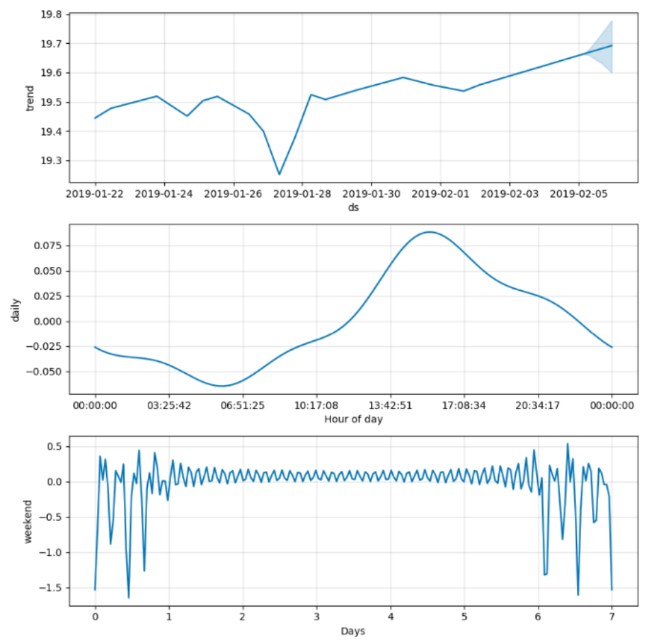
In the sample sequence, the internal temperature trend rises stably until it encounters a weekend, in which the trend will have a shortfall. In the day the internal temperature will fall to the minimum of the day at dawn and in the afternoon it will rise. On the weekend the temperature will be unstable while the weekday temperature is nearly unchanged. In our prediction of internal temperature and energy consumption, the data is generated from the software, therefore the unfixed holiday’s part is off the consideration. The prediction result is as the following figure shows.

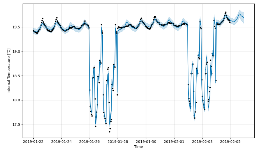
This table shows the performance of the Prophet in different seasons predicting the internal temperature, heating, and cooling energy consumption. It’s clear that the prophet behaves well in winter. This may be the result of the winter having a strong periodicity of internal temperature and heating.

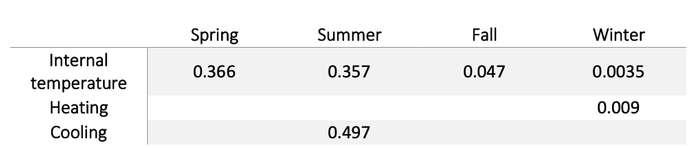
For the Prophet, the greatest advantage of it is its usability. It has acceptable performance when predicting with shortage of data. But if aiming at better accuracy, it will need manual tunning of the trend and periodicity. Another big problem is that the model of the Prophet cannot be fitted twice, which means it cannot add new data and adjust the parameters. It can only use all the data to fit again, consuming extra time for it.