Introduction

The goal of this project is to experiment with predictions using ARIMA models, and in particular to check how the error changes with respect to hyper-parameters.

An ARIMA model is identified by three parameters (p, d, q).

1. p: The number of lag observations included in the model is also called the lag order.

2. d: The number of times that the raw observations are differenced, also called the degree of differencing.

3. q: The size of the moving average window, also called the order of moving average.

Data Processing

In this project, the time series of the number of rentals recorded at each hour in October 2017 is considered in Milano, Munchen of car2go, and Milano of enjoy separately. Before analyzing the data, data cleaning is supposed to be done and the missing data is the major problem that needs to be figured out. Take data of Milano in car2go as an example, there are 710 rental records instead of 720 (24*30) because 10 hours of rental records in October 2017 are missing. In order to feed the data to the ARIMA model, a method must be taken to complement the missing values. In this case, they are replaced with the mean of the records of the same time bin, because the mean value could minimize the consequence of replacing missing data.

Stationary Checking

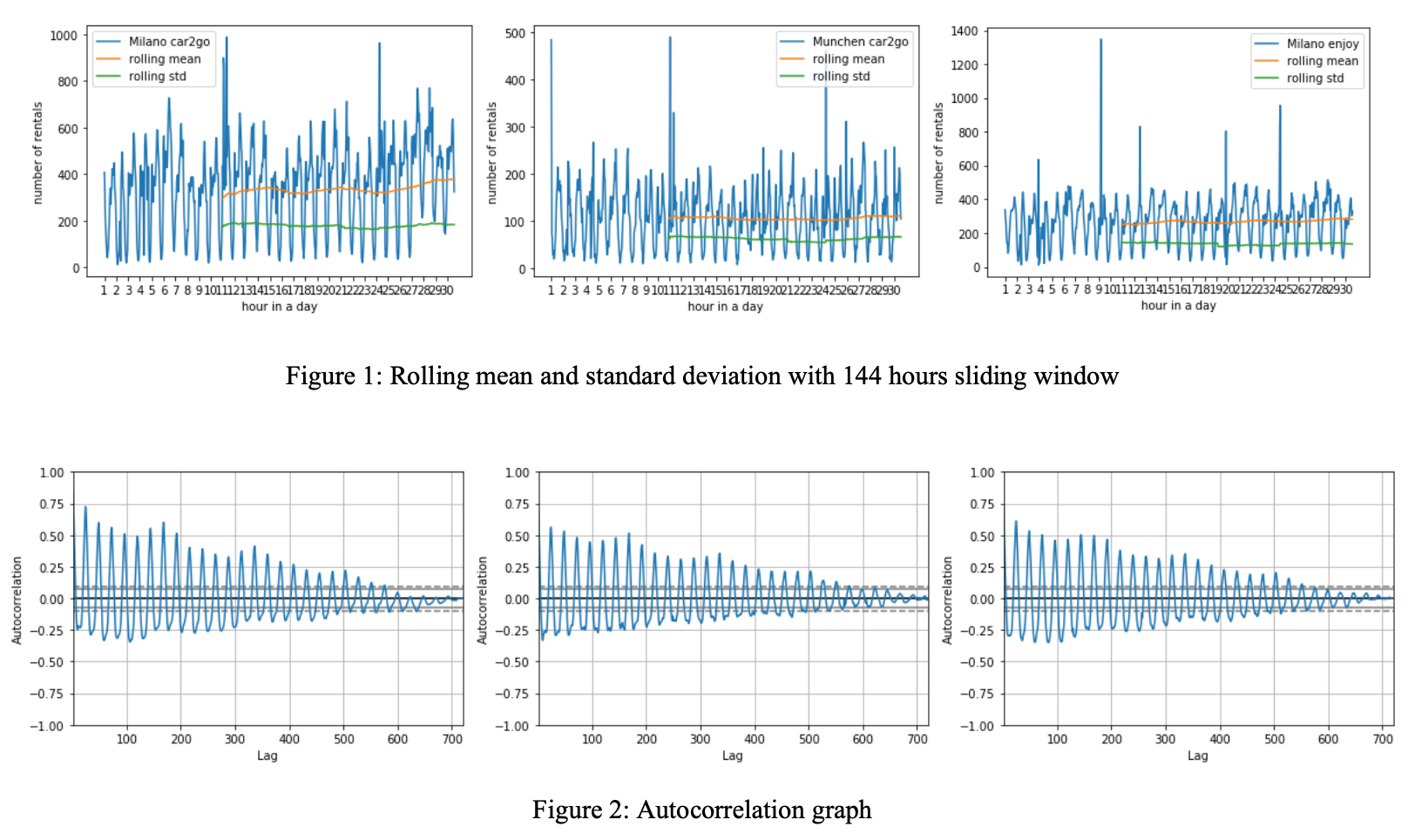
Due to the limitation of the ARIMA model, a stationary series is required for the following steps. In general, a stable time series has no predictable characteristics in the long run. In the rolling plot, a sliding window with a size of 144 hours is chosen because intuitively, the number of rentals will cycle for each week. In the plots, they reflect that this series is stable (Both the mean and the standard are stable). Besides, the oscillation of correlation shows the periodicity of the time series.

Model Specification Choosing

In this step, the ACF (Autocorrelation Function) and the PACF (Partial Autocorrelation Function) of the time series are illustrated, from which it is likely to find possible good values for the hyperparameter ‘p’ (the number of lag observations included in the model) and ‘q’ (the size of the moving average window).

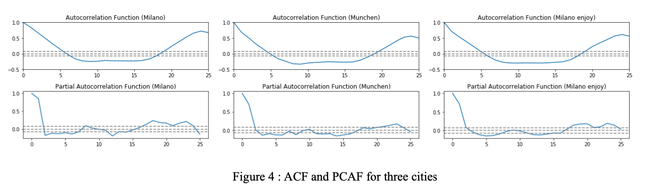
The PACFs show a cut-off at point 1, then the possible value for p is 1. Similarly, the ACFs have tailed off first and cut off after point 4, therefore the candidate value for q is 4. Concerning that the differencing is not used, the hyperparameters of the ARIMA model are (1, 0, 4).

ARIMA model Training

In this study, the train window size will be 1 week and the train policy expanding window, for the rental data may change periodically for each week and the expanding window may improve the accuracy of the model. Thus, the data of the 1st week will be used to train the model and then the model will predict the data in the 2nd week and the differences between the prediction and the true data will be illustrated. For the beginning, the model parameters (p,d,q) are (1, 0, 4).

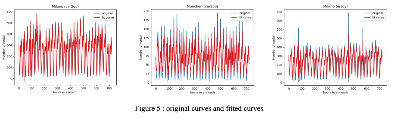
The MSEs are Milano car2go MSE: 3443.3300326919048; Munchen car2go MSE: 476.6718364810478; Milano enjoy MSE: 5054.843662599105.

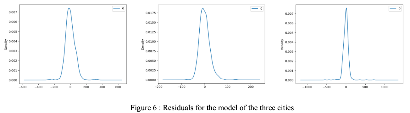
In these three cases, the Munchen data of car2go has the smallest MSE, which can be explained as the good consistency (less outliers) of the data in Munchen. The residuals of the three cities are as follows. The residuals are similar to the uniform distribution, which indicates the effectiveness of the model.